Time-temperature Superposition Fails in a Dramatic Fashion

Temperature dependence of elastic relaxation modulus of a viscoelastic fabric. Here t is the time, Grand is the modulus, and T ₀ < T ₁ < T _two.

Temperature dependence of rubberband modulus of a viscoelastic material under periodic excitation. The frequency is ω, 1000' is the elastic modulus, and T ₀ < T _one < T ₂.

The time–temperature superposition principle is a concept in polymer physics and in the physics of glass-forming liquids.^{[1] [ii] [3] [iv]} This superposition principle is used to determine temperature-dependent mechanical properties of linear viscoelastic materials from known properties at a reference temperature. The elastic moduli of typical amorphous polymers increase with loading rate just decrease when the temperature is increased.^[5] Curves of the instantaneous modulus as a function of time practise not modify shape equally the temperature is changed but appear only to shift left or right. This implies that a primary curve at a given temperature tin can be used equally the reference to predict curves at various temperatures by applying a shift operation. The time-temperature superposition principle of linear viscoelasticity is based on the to a higher place observation.^[6]

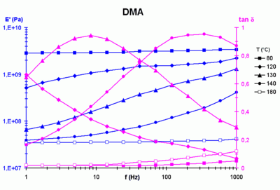
Moduli measured using a dynamic viscoelastic modulus analyzer. The plots show the variation of elastic modulus East′(f, T) and the loss factor, tan δ(f, T), where δ is the stage angle equally a function of frequency f and temperature T.

The application of the principle typically involves the following steps:

• experimental determination of frequency-dependent curves of isothermal viscoelastic mechanical properties at several temperatures and for a small range of frequencies
• computation of a translation factor to correlate these properties for the temperature and frequency range
• experimental determination of a master curve showing the effect of frequency for a broad range of frequencies
• application of the translation cistron to decide temperature-dependent moduli over the whole range of frequencies in the chief curve.

The translation factor is often computed using an empirical relation showtime established by Malcolm L. Williams, Robert F. Landel and John D. Ferry (also called the Williams-Landel-Ferry or WLF model). An culling model suggested by Arrhenius is too used. The WLF model is related to macroscopic motion of the majority material, while the Arrhenius model considers local motion of polymer bondage.

Some materials, polymers in particular, prove a potent dependence of viscoelastic properties on the temperature at which they are measured. If yous plot the elastic modulus of a noncrystallizing crosslinked polymer against the temperature at which you measured information technology, y'all will go a curve which can be divided upward into singled-out regions of physical behavior. At very depression temperatures, the polymer will behave like a glass and exhibit a high modulus. Every bit you lot increase the temperature, the polymer volition undergo a transition from a hard "burnished" country to a soft "rubbery" land in which the modulus tin can be several orders of magnitude lower than it was in the glassy state. The transition from glassy to rubbery behavior is continuous and the transition zone is often referred to every bit the leathery zone. The onset temperature of the transition zone, moving from glassy to rubbery, is known as the glass transition temperature, or T_g.

In the 1940s Andrews and Tobolsky^[7] showed that at that place was a simple relationship between temperature and time for the mechanical response of a polymer. Modulus measurements are made by stretching or compressing a sample at a prescribed rate of deformation. For polymers, irresolute the rate of deformation volition cause the curve described to a higher place to exist shifted forth the temperature centrality. Increasing the rate of deformation volition shift the curve to higher temperatures then that the transition from a glassy to a rubbery land volition happen at higher temperatures.

It has been shown experimentally that the rubberband modulus (Eastward) of a polymer is influenced by the load and the response time. Time–temperature superposition implies that the response fourth dimension function of the elastic modulus at a certain temperature resembles the shape of the aforementioned functions of adjacent temperatures. Curves of E vs. log(response time) at i temperature can be shifted to overlap with next curves, every bit long every bit the data sets did not suffer from ageing effects^[viii] during the test time (see Williams-Landel-Ferry equation).

The Deborah number is closely related to the concept of time-temperature superposition.

Physical principle [edit]

Consider a viscoelastic body that is subjected to dynamic loading. If the excitation frequency is low plenty^[9] the viscous behavior is paramount and all polymer chains take the time to respond to the applied load inside a time period. In dissimilarity, at college frequencies, the chains practice non have the time to fully respond and the resulting bogus viscosity results in an increase in the macroscopic modulus. Moreover, at constant frequency, an increase in temperature results in a reduction of the modulus due to an increase in free volume and chain motion.

Time–temperature superposition is a process that has get important in the field of polymers to observe the dependence upon temperature on the modify of viscosity of a polymeric fluid. Rheology or viscosity can oft be a stiff indicator of the molecular structure and molecular mobility. Time–temperature superposition avoids the inefficiency of measuring a polymer's behavior over long periods of fourth dimension at a specified temperature by utilizing the fact that at higher temperatures and shorter time the polymer will behave the aforementioned, provided in that location are no stage transitions.

Time-temperature superposition [edit]

Schematic of the development of the instantaneous modulus East(t,T) in a static relaxation test. t is the fourth dimension and T is the temperature.

Consider the relaxation modulus E at two temperatures T and T ₀ such that T > T ₀. At constant strain, the stress relaxes faster at the higher temperature. The principle of time-temperature superposition states that the change in temperature from T to T ₀ is equivalent to multiplying the time scale by a constant gene a _T which is just a part of the two temperatures T and T ₀. In other words,

${\displaystyle E(t,T)=E({\frac {t}{a_{\rm {T}}}},T_{0})\,.}$

The quantity a _T is called the horizontal translation factor or the shift factor and has the properties:

${\displaystyle {\begin{aligned}&T<T_{0}\quad \implies \quad a_{\rm {T}}<1\\&T>T_{0}\quad \implies \quad a_{\rm {T}}>one\\&T=T_{0}\quad \implies \quad a_{\rm {T}}=i\,.\end{aligned}}}$

The superposition principle for complex dynamic moduli (K* = G' + i G'' ) at a stock-still frequency ω is obtained similarly:

${\displaystyle {\begin{aligned}G'(\omega ,T)&=G'\left(a_{\rm {T}}\,\omega ,T_{0}\right)\\Thou''(\omega ,T)&=G''\left(a_{\rm {T}}\,\omega ,T_{0}\right).\end{aligned}}}$

A decrease in temperature increases the fourth dimension characteristics while frequency characteristics decrease.

Human relationship betwixt shift factor and intrinsic viscosities [edit]

For a polymer in solution or "molten" country the following relationship can be used to determine the shift factor:

${\displaystyle a_{\rm {T}}={\frac {\eta _{\rm {T}}}{\eta _{\rm {T0}}}}}$

where η _T0 is the viscosity (not-Newtonian) during continuous flow at temperature T ₀ and η _T is the viscosity at temperature T.

The time–temperature shift gene can besides be described in terms of the activation energy (E _a). By plotting the shift factor a _T versus the reciprocal of temperature (in 1000), the slope of the curve tin be interpreted as E _a/k, where k is the Boltzmann constant = 8.64x10⁻⁵ eV/K and the activation energy is expressed in terms of eV.

Shift factor using the Williams-Landel-Ferry (WLF) model [edit]

Curve of the variation of a _T every bit a role of T for a reference temperature T ₀.^[10]

The empirical human relationship of Williams-Landel-Ferry,^[11] combined with the principle of fourth dimension-temperature superposition, tin can business relationship for variations in the intrinsic viscosity η ₀ of baggy polymers as a function of temperature, for temperatures about the glass transition temperature T _g. The WLF model also expresses the change with the temperature of the shift factor.

Williams, Landel and Ferry proposed the following human relationship for a _T in terms of (T-T ₀) :

${\displaystyle \log a_{\rm {T}}=-{\frac {C_{1}(T-T_{0})}{C_{2}+(T-T_{0})}}}$

where ${\displaystyle \log }$ is the decadic logarithm and C ₁ and C ₂ are positive constants that depend on the textile and the reference temperature. This human relationship holds only in the gauge temperature range [T_k, T_k + 100 °C]. To determine the constants, the factor a _T is calculated for each component M′ and 1000 of the complex measured modulus M*. A proficient correlation between the 2 shift factors gives the values of the coefficients C _i and C ₂ that narrate the material.

If T ₀ = T _g:

${\displaystyle \log a_{\rm {T}}=-{\frac {C_{1}^{k}(T-T_{m})}{C_{2}^{grand}+(T-T_{yard})}}=\log \left({\frac {\eta _{\rm {T}}}{\eta _{T_{thousand}}}}\right)}$

where C ^g _i and C ¹⁰⁰⁰ _two are the coefficients of the WLF model when the reference temperature is the drinking glass transition temperature.

The coefficients C ₁ and C ₂ depend on the reference temperature. If the reference temperature is changed from T ₀ to T′ ₀, the new coefficients are given by

${\displaystyle C'_{one}={\frac {C_{i}\,C_{2}}{C_{2}+(T'_{0}-T_{0})}}\qquad {\rm {and}}\qquad C'_{2}=C_{2}+(T'_{0}-T_{0})\,.}$

In particular, to transform the constants from those obtained at the glass transition temperature to a reference temperature T ₀,

${\displaystyle C_{1}^{0}={\frac {C_{1}^{thou}\,C_{2}^{yard}}{C_{two}^{thou}+(T_{0}-T_{g})}}\qquad {\rm {and}}\qquad C_{2}^{0}=C_{2}^{thou}+(T_{0}-T_{g})\,.}$

These same authors have proposed the "universal constants" C ^g ₁ and C ^g ₂ for a given polymer system exist collected in a tabular array. These constants are approximately the same for a large number of polymers and can be written C ^chiliad ₁ ≈ 15 and C ^g _ii ≈ fifty M. Experimentally observed values deviate from the values in the table. These orders of magnitude are useful and are a practiced indicator of the quality of a relationship that has been computed from experimental information.

Structure of main curves [edit]

Master curves for the instantaneous modulus E′ and the loss gene tanδ as a function of frequency. The data accept been fit to a polynomial of degree 7.

The principle of time-temperature superposition requires the assumption of thermorheologically unproblematic behavior (all curves have the same characteristic time variation law with temperature). From an initial spectral window [ω ₁, ω ₂] and a series of isotherms in this window, nosotros can calculate the master curves of a material which extends over a broader frequency range. An arbitrary temperature T ₀ is taken equally a reference for setting the frequency scale (the curve at that temperature undergoes no shift).

In the frequency range [ω _ane, ω _two], if the temperature increases from T ₀, the complex modulus Due east′(ω) decreases. This amounts to explore a role of the chief curve respective to frequencies lower than ω _one while maintaining the temperature at T ₀. Conversely, lowering the temperature corresponds to the exploration of the part of the curve respective to high frequencies. For a reference temperature T ₀, shifts of the modulus curves have the aamplitude log(a _T). In the area of glass transition, a _T is described by an homographic function of the temperature.

The viscoelastic behavior is well modeled and allows extrapolation beyond the field of experimental frequencies which typically ranges from 0.01 to 100 Hz .

Principle of construction of a master curve for E′ for a reference temperatureT ₀. f=ω is the frequency. The shift factor is computed from information in the frequency range ω ₁ = one Hz and ω ₂ = chiliad Hz.

Shift factor using Arrhenius law [edit]

The shift factor (which depends on the nature of the transition) tin can be defined, below T _thousand, ^{[ commendation needed ]} using an Arrhenius law:

${\displaystyle \log(a_{\rm {T}})=-{\frac {E_{a}}{two.303R}}\left({\frac {1}{T}}-{\frac {1}{T_{0}}}\right)}$

where E _a is the activation energy, R is the universal gas constant, and T ₀ is a reference temperature in kelvins. This Arrhenius law, under this glass transition temperature, applies to secondary transitions (relaxation) called β-transitions.

Limitations [edit]

For the superposition principle to apply, the sample must exist homogeneous, isotropic and amorphous. The material must be linear viscoelastic nether the deformations of involvement, i.e., the deformation must exist expressed every bit a linear function of the stress past applying very small strains, eastward.g. 0.01%.

To apply the WLF relationship, such a sample should be sought in the gauge temperature range [T _yard, T _g + 100 °C], where α-transitions are observed (relaxation). The study to determine a _T and the coefficients C ₁ and C _two requires extensive dynamic testing at a number of scanning frequencies and temperature, which represents at least a hundred measurement points.

Time-temperature-plasticization superposition [edit]

In 2019, time-temperature superposition principle was extended to include the effect of plasticization. The extended principle, termed fourth dimension-temperature-plasticization superposition principle (TTPSP), was described by Krauklis et al.^[12] Using this principle, Krauklis et al. obtained a main bend for the creep compliance of a dry and plasticized (saturated with h2o) amine-based epoxy.

The extended methodology enables prediction of long-term viscoelastic behavior of plasticized baggy polymers at temperatures beneath the glass transition temperatures T _g based on the short-term creep experimental data of the respective dry out material and the difference between T _g values of dry out and plasticized polymer. Furthermore, the T _g of the plasticized epoxy can be predicted with reasonable accuracy using the T _g of the dry material (T _{g dry}) and the shift gene due to plasticization (log a _dry-to-plast).

References [edit]

1. ^ Hiemenz, Paul C.; Social club, Timothy P. (2007). Polymer chemical science (2nd ed.). Taylor & Francis. pp. 486–491. ISBN1574447793.
2. ^ Li, Rongzhi (Feb 2000). "Fourth dimension-temperature superposition method for drinking glass transition temperature of plastic materials". Materials Science and Engineering: A. 278 (one–ii): 36–45. doi:10.1016/S0921-5093(99)00602-4.
3. ^ van Gurp, Marnix; Palmen, Jo (Jan 1998). "Time-temperature superposition for polymeric blends" (PDF). Rheology Message. 67 (1): 5–8. Retrieved 7 December 2021.
4. ^ Olsen, Niels Boye; Christensen, Tage; Dyre, Jeppe C. (2001). "Time-Temperature Superposition in Viscous Liquids". Physical Review Letters. 86 (7): 1271–1274. arXiv:cond-mat/0006165. Bibcode:2001PhRvL..86.1271O. doi:10.1103/PhysRevLett.86.1271. ISSN 0031-9007. PMID 11178061.
5. ^ Experiments that determine the mechanical properties of polymers ofttimes use periodic loading. For such situations, the loading rate is related to the frequency of the practical load.
6. ^ Christensen, Richard M. (1971). Theory of viscoelasticity: an introduction. New York: Bookish Press. p. 92. ISBN0121742504.
7. ^ Andrews, R. D.; Tobolsky, A. 5. (August 1951). "Elastoviscous properties of polyisobutylene. Four. Relaxation time spectrum and calculation of bulk viscosity". Periodical of Polymer Scientific discipline. 7 (23): 221–242. doi:10.1002/political leader.1951.120070210.
8. ^ Struik, L. C. East. (1978). Concrete aging in baggy polymers and other materials. Amsterdam: Elsevier Scientific Pub. Co. ISBN9780444416551.
9. ^ For the superposition principle to apply, the excitation frequency should be well above the feature time τ (too called relaxation fourth dimension) which depends on the molecular weight of the polymer.
10. ^ Curve has been generated with information from a dynamic examination with a double scanning frequency / temperature on a viscoelastic polymer.
11. ^ Ferry, John D. (1980). Viscoelastic backdrop of polymers (3d ed.). New York: Wiley. ISBN0471048941.
12. ^ Krauklis, A. E.; Akulichev, A. G.; Gagani, A. I.; Echtermeyer, A. T. (2019). "Time–Temperature–Plasticization Superposition Principle: Predicting Creep of a Plasticized Epoxy". Polymers. 11 (11): 1848–1859. doi:x.3390/polym11111848. PMC6918382. PMID 31717515.

Meet besides [edit]

• Viscoelasticity
• Temperature dependence of liquid viscosity
• Williams-Landel-Ferry equation

Share this post